WWC effect size omega factor (to adjust for n) and R sample

https://ies.ed.gov/ncee/wwc/Docs/referenceresources/WWC_Procedures_Handbook_V4_1_Draft.pdf

See Page 16.

two_values<-view1b[3:4]
num<-view1b[2]

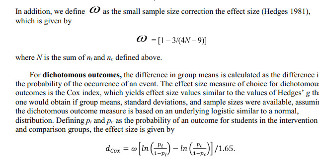
omega<-(1-3/(4*num-9))

C_LOGIT<-two_values[1]
C_EXP<-exp(C_LOGIT)/(1+exp(C_LOGIT))
C_ODDS<-C_EXP/(1-C_EXP)
C_STEP1<-log(C_ODDS)
T_LOGIT<-two_values[1]+two_values[2]
T_EXP<-exp(T_LOGIT)/(1+exp(T_LOGIT))
T_ODDS<-T_EXP/(1-T_EXP)
T_STEP1<-log(T_ODDS)
STEP2<-T_STEP1-C_STEP1
wwc_effect_size<-STEP2/1.65

wwc_effect_size_omega<-(omega*STEP2)/1.65

odds_ratio<-T_ODDS/C_ODDS


How to create a bar graph off logistic regression results

This is how you can create a graph comparing the treatment group and the comparison group's %s  -- based on findings from the logistic regression model.

Based on the final multivariate model, you get the program effect in logit. For example:

-0.223

You also run the simpler model with the treatment program indicator only. Get the intercept value. For example:

1.7081

When this logic is converted into a %, it will be the unadjusted % of the comparison group.

Use these two numbers to derive %s for the treatment group and comparison group.

https://docs.google.com/spreadsheets/d/0B7AoA5fyqX_sN0RUc0E5aFowb00/edit?usp=sharing&ouid=116965977650967783537&resourcekey=0-nGn3k4fyPrVKP2f4Xm-fOA&rtpof=true&sd=true

The resulting graph fixes the % of the comparison group to the simple % of the comparison group and shows the % of the treatment group based on the program effect adjusted for covariates.

If you use the intercept value and the program effect value from the final multivariate model, the meaning of percentages become non-intuitive. If you center predictors (except for the treatment indicator), the intercept will represent a typical person in the dataset. But this is a bit difficult to undestand.

Without centering, the intercept value will represent someone who is, for example, female, white, etc., depending on omitted categories of the variables. If continuous variables are included and if the value of 0 in that variable is not intuitive, the meaning of the intercept is a difficult to interpret.

I recommend using the intercept from the simple model (only the treatment group is the predictor), so the comparison group % will be fixed at a simple descriptive % of the comparison group.


SAS data variable function detepart

if datepart(OffenseDate) > s_date;


data crim;
set abc.crim_history;
format new_date MMDDYY10.;
format s_date MMDDYY10.;
new_date=datepart(OffenseDate);
s_date=mdy(1,1,2019);
instruction="Drop ";
if new_date > s_date then instruction="Keep";
*if datepart(OffenseDate) > s_date;
run;

#clear console
rm(list = ls())

setwd("C:/sas/(01) D/newdata")

crim<- read_excel("HistoryCombined.xlsx",sheet="History ")

#Creating the new dataset after WV review -- I added dual credit info per grade level
write.foreign(crim, "C:/sas/(01) D/newdata/data.txt",
"C:/sas/(01) D/newdata/data.sas", package="SAS")


Packages I use are:

library(broom)
library(compute.es)
library(dplyr)
library(forcats)
library(FSA)
library(gapminder)
library(ggplot2)
library(gmodels)
library(haven)
library(here)
library(leaflet)
library(magrittr)
library(markdown)
library(MatchIt)
library(plyr)
library(psych)
library(purrr)
library(readr)
library(readxl)
library(sas7bdat)
library(sf)
library(sqldf)
library(stringr)
library(summarytools)
library(tidyverse)
library(tmap)
library(tmaptools)
library(descr)
library(MatchIt)
library(sjmisc)
library(writexl)
library(skimr)
library(lme4)
library(lmerTest)
library(car)
library(foreign)

Logistic regression in R and creating WWC effect size

#https://stats.oarc.ucla.edu/r/dae/logit-regression/
mylogit1 <- glm(enroll_FR_spring ~ treat+ male +minority +disadv +binary_dualcredit+SAT_TOTAL + GPA_12_GRADE +FALL_2020_INSTNAME, data = sample, family = "binomial")
summary(mylogit1)

coef_table<-(coef(mylogit1))
two_values<-coef_table[1:2]
C_LOGIT<-two_values[1]
C_EXP<-exp(C_LOGIT)/(1+exp(C_LOGIT))
C_ODDS<-C_EXP/(1-C_EXP)
C_STEP1<-log(C_ODDS)
T_LOGIT<-two_values[1]+two_values[2]
T_EXP<-exp(T_LOGIT)/(1+exp(T_LOGIT))
T_ODDS<-T_EXP/(1-T_EXP)
T_STEP1<-log(T_ODDS)
STEP2<-T_STEP1-C_STEP1
wwc_effect_size<-STEP2/1.65
odds_ratio<-T_ODDS/C_ODDS

R function example -- when a data frame is involved

var.labels = c(age="Age in Years", GPA_12_GRADE="Test Score", gpa="GPA", sex="Sex of the participant")
DATA_KAZ <- data.frame(age = c(21, 30, 25, 41, 29, 33,NA),
GPA_12_GRADE = c(75, 65, 88, 92, 97, 79, 83),
gpa = c(3.4,2.7,3.9,4.0,2.5,1.2, 3.2),
sex = factor(c(1, 2, 1, 2, 1, 2, 1), labels = c("Female", "Male")),
race=factor(c(1,1,2,2,3,3, 1), labels = c("White", "Black","Hispanic")))
label(DATA_KAZ) = as.list(var.labels[match(names(DATA_KAZ), names(var.labels))])

CCC<-filter(DATA_KAZ,sex=="Female")
TTT<-filter(DATA_KAZ,sex=="Male")


kaz_macro<-function(kaz1){
col_name <- deparse(substitute(kaz1))
C_mean<-mean(CCC[[col_name]])
T_mean<-mean(TTT[[col_name]])
C_sd<-sd(CCC[[col_name]])
T_sd<-sd(TTT[[col_name]])
C_n<-length(CCC[[col_name]])
T_n<-length(TTT[[col_name]])

simple_gap=T_mean-C_mean
g1<- ((T_n-1)*(T_sd*T_sd))+((C_n-1)*(C_sd*C_sd))
g2= T_n + C_n -2
g3= sqrt(g1/g2)
wwc_effect= simple_gap/g3
wwc_effect
}
kaz_macro(GPA_12_GRADE)
kaz_macro(gpa)